Molden examples
Running the following input of positronic glycine
SYSTEM_DESCRIPTION='Gly.e+-molden'

GEOMETRY
e-(N) 6-311G     0.851078    0.379034    0.538699
e-(C) 6-311G     0.011668   -0.714576    1.101899
e-(C) 6-311G     0.016098   -0.668656    2.636109
e-(O) 6-311G     0.714088    0.201754    3.154209
e-(O) 6-311G    -0.685842   -1.520986    3.175689
e-(H) 6-311G     1.816418    0.263714    0.801099
e-(H) 6-311G     0.409998   -1.655016    0.751139
e-(H) 6-311G    -0.992842   -0.593136    0.726189
e-(H) 6-311G     0.527967    1.271782    0.883152
e-(H) 6-311G     0.787819    0.376813   -0.469282
e+ PSX-TZ        0.714088    0.201754    3.154209
e+ PSX-TZ       -0.685842   -1.520986    3.175689 addParticles=-1
N dirac          0.851078    0.379034    0.538699
C dirac          0.011668   -0.714576    1.101899
C dirac          0.016098   -0.668656    2.636109
O dirac          0.714088    0.201754    3.154209
O dirac         -0.685842   -1.520986    3.175689
H dirac          1.816418    0.263714    0.801099
H dirac          0.409998   -1.655016    0.751139
H dirac         -0.992842   -0.593136    0.726189
H dirac          0.527967    1.271782    0.883152
H dirac          0.787819    0.376813   -0.469282
END GEOMETRY

TASKS
	method = "RHF"
END TASKS

OUTPUTS
	moldenFile
END OUTPUTS
Produces two molden files, one for the electrons and one for the positron, their filenames are provided in the output.
 --------------------------------------------------------
 MOLDENFILE             1
                   for all species
          FileName: Gly.e+-molden.E-.molden
          FileName: Gly.e+-molden.E+.molden
 --------------------------------------------------------
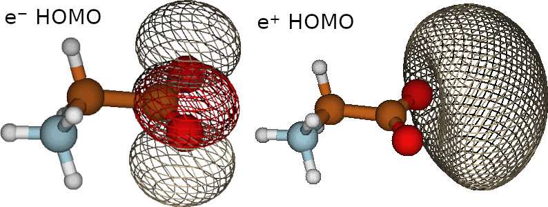
These files contain the the electronic and positronic orbitals. We can visualize these orbitals using the molden software (https://www.theochem.ru.nl/molden/ ), as observed in the following figure
Localized orbitals and fchk files
Localized orbitals are generated with the Erkale software (https://github.com/susilehtola/erkale ), adding the following lines in the CONTROL block
SYSTEM_DESCRIPTION='Gly.e+-localize-molden'

GEOMETRY
e-(N) 6-311G     0.851078    0.379034    0.538699
e-(C) 6-311G     0.011668   -0.714576    1.101899
e-(C) 6-311G     0.016098   -0.668656    2.636109
e-(O) 6-311G     0.714088    0.201754    3.154209
e-(O) 6-311G    -0.685842   -1.520986    3.175689
e-(H) 6-311G     1.816418    0.263714    0.801099
e-(H) 6-311G     0.409998   -1.655016    0.751139
e-(H) 6-311G    -0.992842   -0.593136    0.726189
e-(H) 6-311G     0.527967    1.271782    0.883152
e-(H) 6-311G     0.787819    0.376813   -0.469282
e+ PSX-TZ        0.714088    0.201754    3.154209
e+ PSX-TZ       -0.685842   -1.520986    3.175689 addParticles=-1
N dirac          0.851078    0.379034    0.538699
C dirac          0.011668   -0.714576    1.101899
C dirac          0.016098   -0.668656    2.636109
O dirac          0.714088    0.201754    3.154209
O dirac         -0.685842   -1.520986    3.175689
H dirac          1.816418    0.263714    0.801099
H dirac          0.409998   -1.655016    0.751139
H dirac         -0.992842   -0.593136    0.726189
H dirac          0.527967    1.271782    0.883152
H dirac          0.787819    0.376813   -0.469282
END GEOMETRY

TASKS
	method = "RHF"
END TASKS

CONTROL
	localizeOrbitals=.T.
	erkaleLocalizationMethod="MU"
END CONTROL

OUTPUTS
	moldenFile
END OUTPUTS
Here with “MU” we selected the Pipek-Mozay localization scheme using Mulliken charges. Check Erkale manual for a full list of the localization procedures available. To transfer the orbitals to Erkale, openLowdin generates fchk files. In the output, you will find the Erkale localization log.
 --------------------------------------------------------
            FCHKFILE    1
   for all species
          FileName: Gly.e+-localize-molden.E-.fchk
          FileName: Gly.e+-localize-molden.E+.fchk
 --------------------------------------------------------

  ERKALE ORBITAL LOCALIZATION
 ==============================

ERKALE - Localization from Hel, serial version.
(c) Susi Lehtola, 2010-2016.

[...]

Localizing orbitals: 1 2 3 4 5 6 7 8 9 10 11 12 13 14 15 16 17 18 19 20
Initializing generalized Pipek-Mezey calculation with Mulliken charges... done.
Initialization of Pipek-Mezey took 0.00 s
  iter              J        delta J         <G,G>
     1   1.154017e+01   1.517727e+00  1.174829e+00   0.00 s
     2   1.274872e+01   1.208552e+00  1.673368e+00   0.00 s
[...]
    89   1.576852e+01   7.696281e-09  5.667527e-09   0.00 s
Converged.
Localization done in 0.06 s.
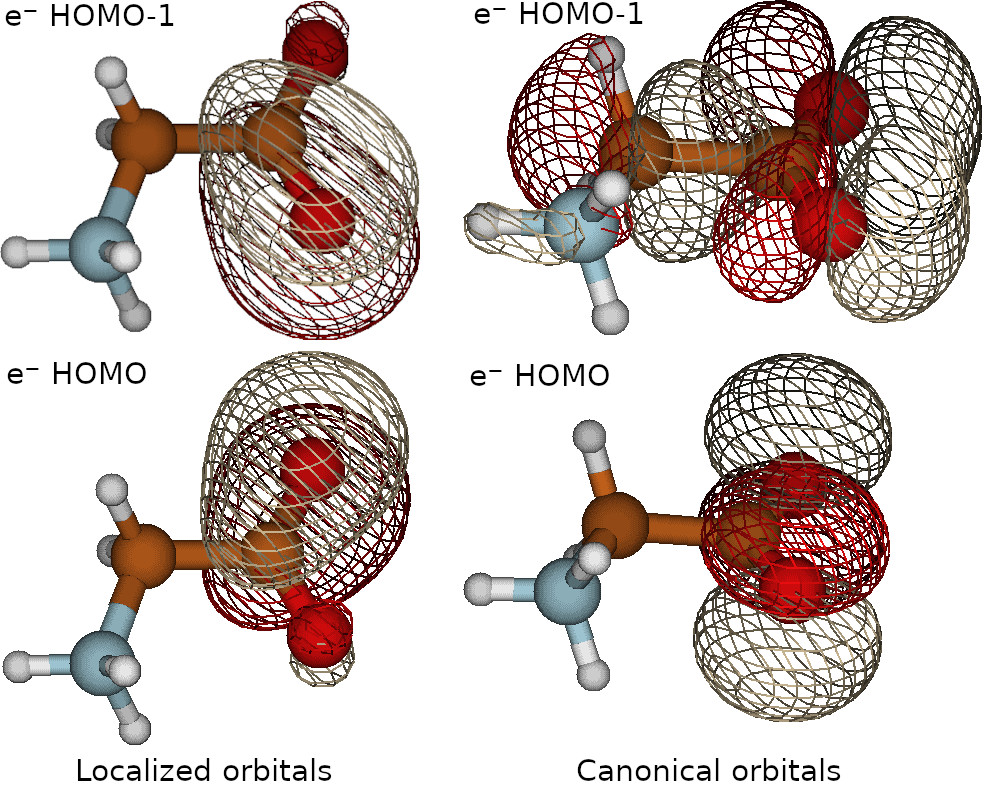
For this example, the localization procedure only affects the electronic orbitals, because there is only a single positronic orbital. When localized orbitals are requested, openlowdin will generate the molden files with them. Check in the following figure a comparison between the non-localized (right) and localized (left) HOMO of positronic glycine
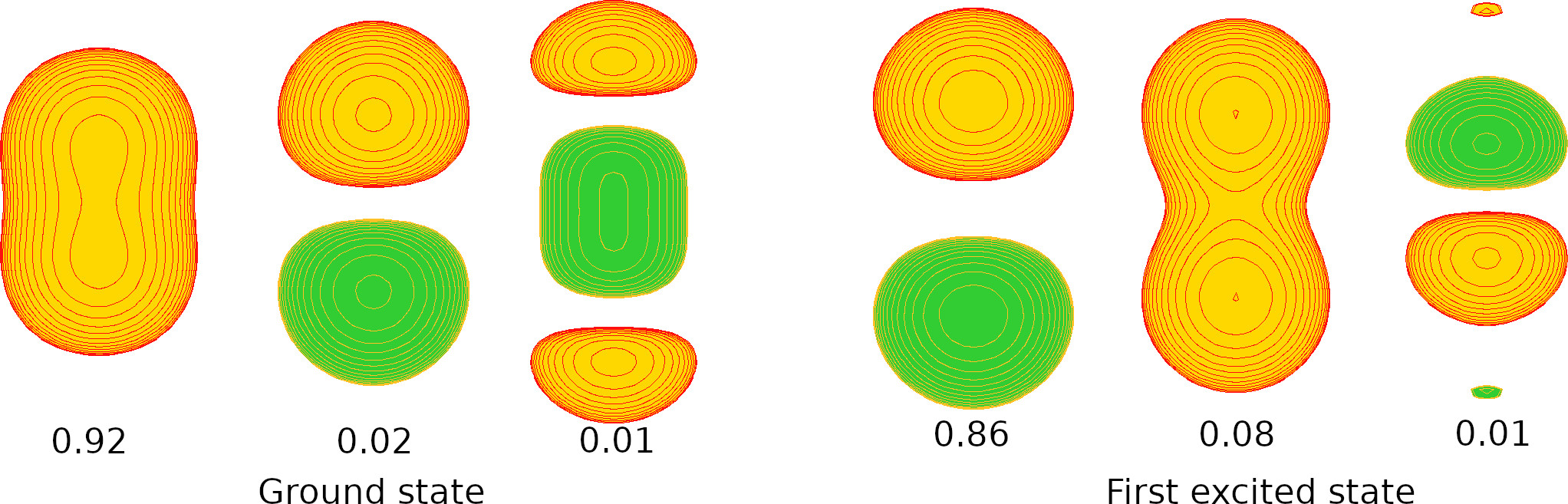
CI excited states
When we run a configuration interaction calculation we can generate molden files for the excited states. For example, in the Positron covalent bond (e+H-H-.CISDTQ-DZ.lowdin) example we added “state=2” to get the natural orbitals of the first excited state. In the output of that calculation we find
   We are printing molden files for the CI states!
 --------------------------------------------------------
          MOLDENFILE    1
   for all species
          FileName: e+H-H-.CISDTQ-DZ.E-ALPHA.molden
          FileName: e+H-H-.CISDTQ-DZ.E-BETA.molden
          FileName: e+H-H-.CISDTQ-DZ.E+.molden
 --------------------------------------------------------

   We are printing molden files for the CI states!
 --------------------------------------------------------
          MOLDENFILE    2
   for all species
 for excited state:     2
          FileName: e+H-H-.CISDTQ-DZ.E-ALPHA-s2.molden
          FileName: e+H-H-.CISDTQ-DZ.E-BETA-s2.molden
          FileName: e+H-H-.CISDTQ-DZ.E+-s2.molden
 --------------------------------------------------------
In the following figure we plot the positronic natural orbitals with the highest contributions to the ground (right) and first excited (left) states