Cubes examples

With openLowdin, we can generate orbital and density Gaussian cube files (https://h5cube-spec.readthedocs.io/en/latest/cubeformat.html ). Here we present an example for positronic formate

SYSTEM_DESCRIPTION='Positronic formate' 

GEOMETRY
e-(C) cc-pVDZ		0.0000000	0.0000000	0.3157740
e-(H) cc-pVDZ		0.0000000	0.0000000	1.4510170
e-(O) aug-cc-pVDZ	0.0000000	1.1357680	-0.2091040
e-(O) aug-cc-pVDZ	0.0000000	-1.1357680	-0.2091040 addParticles=1
e+    PSX-DZ		0.0000000	1.1357680	-0.2091040
e+    PSX-DZ		0.0000000	-1.1357680	-0.2091040 addParticles=-1
C     dirac		0.0000000	0.0000000	0.3157740
H     dirac		0.0000000	0.0000000	1.4510170
O     dirac		0.0000000	1.1357680	-0.2091040
O     dirac		0.0000000	-1.1357680	-0.2091040
END GEOMETRY

TASKS
	method = "RHF"
END TASKS

OUTPUTS
	densityCube  cubeSize=5  point1=0.0 0.0 0.0 species="E-" pointsPerDim=100
	densityCube  cubeSize=20  point1=0.0 0.0 -2.5 species="E+" pointsPerDim=50
	orbitalCube  cubeSize=15  center=0.0 0.0 -2.5 species="ALL" scanStep=0.5
	orbitalCube  cubeSize=10  center=0.0 0.0 0.0 species="E-" orbital=11 scanStep=0.25
END OUTPUTS

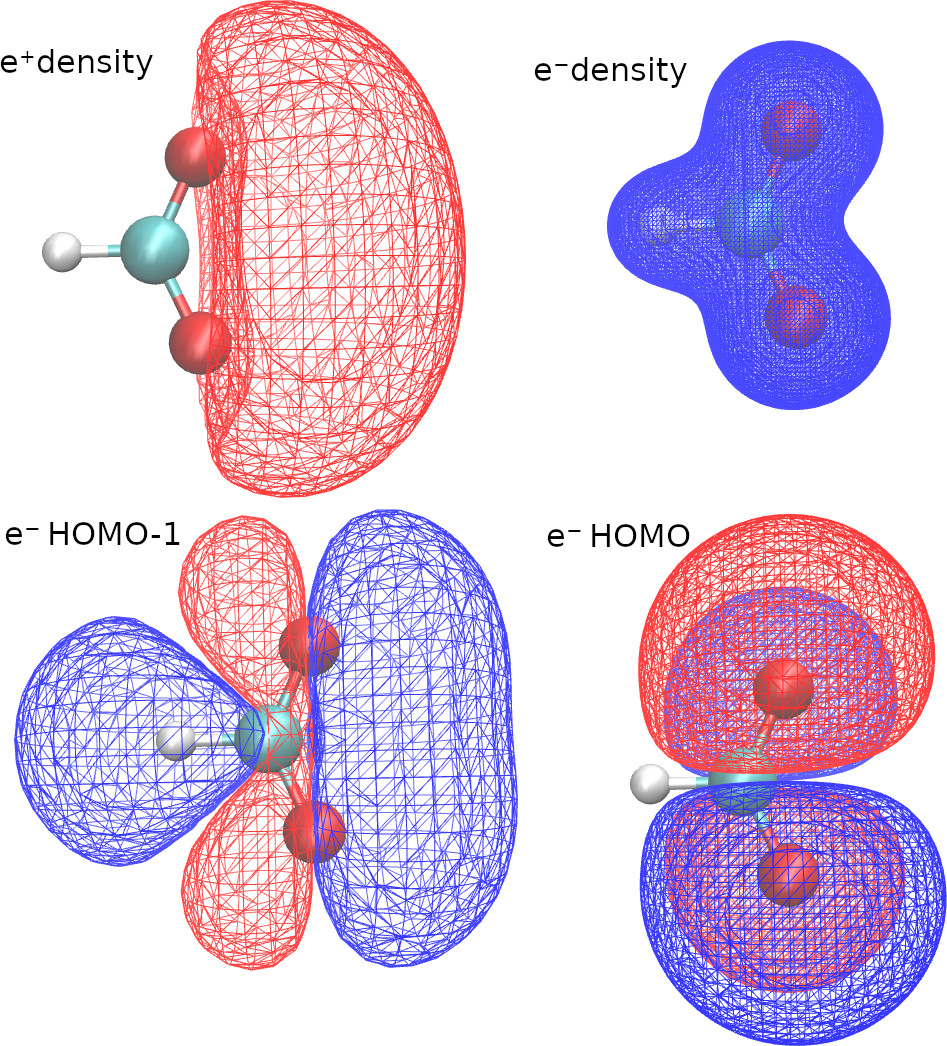
With the first two lines in the OUTPUTS block, we request density cubes for electrons and positrons. Here, we use a different size for each cube, because the positronic density is more delocalized.

With the last two lines of the OUTPUTS block, we request orbitals cubes. When we select “species”=”ALL”, openLowdin will generate a cube with the HOMO of each species. We can also select a specific orbital, by selecting a species and an orbital number. In this example we requested the HOMO-1 of the formate anion.

We pass the option “center” or “point1” to define the origin of the cube, and we use the “pointsPerDim” or the “scanStep” options to adjust its resolution. “scanStep” sets the separation between grid points, whereas “pointsPerDim=N” sets the total number of points per side, such that the number of points in the cube is N³.

Therefore, running this calculation produces five cube files, with the filenames provided in the output.

 --------------------------------------------------------
         DENSITYCUBE    1
       for species: E-
  cube size (a.u.):    9.44863
cube center (a.u.):    0.00000   0.00000   0.00000
         No. steps:        100       100       100
          FileName: HCOOPs.HF.densOrbCube.E-.dens.cub                                                                   
 --------------------------------------------------------
 
 --------------------------------------------------------
         DENSITYCUBE    2
       for species: E+
  cube size (a.u.):   37.79452
cube center (a.u.):    0.00000   0.00000  -4.72432
         No. steps:         50        50        50
          FileName: HCOOPs.HF.densOrbCube.E+.dens.cub                                                                   
 --------------------------------------------------------
 
 --------------------------------------------------------
         ORBITALCUBE    3
   for all species  
        for the highest occupied orbital
  cube size (a.u.):   28.34589
cube center (a.u.):    0.00000   0.00000  -4.72432
         No. steps:         60        60        60
          FileName: HCOOPs.HF.densOrbCube.E-.orb12.cub                                                                  
          FileName: HCOOPs.HF.densOrbCube.E+.orb1.cub                                                                   
 --------------------------------------------------------
 
 --------------------------------------------------------
         ORBITALCUBE    4
       for species: E-
       for orbital:         11
  cube size (a.u.):   18.89726
cube center (a.u.):    0.00000   0.00000   0.00000
         No. steps:         80        80        80
          FileName: HCOOPs.HF.densOrbCube.E-.orb11.cub                                                                  
 --------------------------------------------------------

The VMD software (https://www.ks.uiuc.edu/Research/vmd/ ) is an excellent tool to visualize the cube files. Here are some VMD plots obtained from the positronic formate cubes

We can also request cubes for localized orbitals. The keywords required are identical to those employed in the Molden examples.

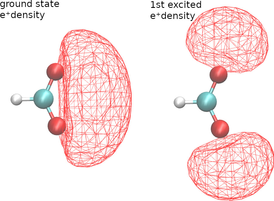
Excited states

For configuration interaction calculations, we can generate cubes for excited state natural orbitals and excited state densities. For example, with the following CI singles calculation,

SYSTEM_DESCRIPTION='Positronic formate'

GEOMETRY
e-(C) cc-pVDZ           0.0000000       0.0000000       0.3157740
e-(H) cc-pVDZ           0.0000000       0.0000000       1.4510170
e-(O) aug-cc-pVDZ       0.0000000       1.1357680       -0.2091040
e-(O) aug-cc-pVDZ       0.0000000       -1.1357680      -0.2091040 addParticles=1
e+    PSX-DZ            0.0000000       1.1357680       -0.2091040
e+    PSX-DZ            0.0000000       -1.1357680      -0.2091040 addParticles=-1
C     dirac             0.0000000       0.0000000       0.3157740
H     dirac             0.0000000       0.0000000       1.4510170
O     dirac             0.0000000       1.1357680       -0.2091040
O     dirac             0.0000000       -1.1357680      -0.2091040
END GEOMETRY

TASKS
     	method = "UHF"
	configurationInteractionLevel="CIS"
END TASKS

CONTROL
	numberOfCIstates=2
	CIstatesToPrint=2
END CONTROL

OUTPUTS
	densityCube  cubeSize=20  point1=0.0 0.0 -2.5 species="E+" pointsPerDim=50 state=1
	densityCube  cubeSize=20  point1=0.0 0.0 -2.5 species="E+" pointsPerDim=50 state=2
END OUTPUTS

we get the ground and first-excited state positronic densities.